Introduction
This article is going to walk through building a model to predict football results using the Poisson distribution. As we'll find out, the model is fairly simplistic and struggles at points. However, it provides us a with great base to improve from over the next few articles in this series.
Let's get started!
The Data
Our model will work by predicting the number of goals scored / conceded by each team when they play each other based on their historical performances. To work that out we're going to need some data so let's grab some football results from the awesome football-data.co.uk website.
import pandas as pd

df = pd.read_csv("https://www.football-data.co.uk/mmz4281/1718/E0.csv")
df[["Date", "HomeTeam", "AwayTeam", "FTHG", "FTAG"]].head()
| Date | HomeTeam | AwayTeam | FTHG | FTAG | |
|---|---|---|---|---|---|
| 0 | 11/08/2017 | Arsenal | Leicester | 4 | 3 |
| 1 | 12/08/2017 | Brighton | Man City | 0 | 2 |
| 2 | 12/08/2017 | Chelsea | Burnley | 2 | 3 |
| 3 | 12/08/2017 | Crystal Palace | Huddersfield | 0 | 3 |
| 4 | 12/08/2017 | Everton | Stoke | 1 | 0 |
We've now got the team names, the number of goals scored by the home team (FTHG) at full time and the number of goals scored by the away team (FTAG) at full time, which is everything we need to get started.
Home Advantage
Let's dig into the data to get a better understanding of what we're trying to model. We'll start off simple by looking at the average goals scored.
df[["FTHG", "FTAG"]].mean()
FTHG    1.531579
FTAG    1.147368
dtype: float64
On average, the home team scores around a third of a goal more than the away team so to it looks like our model will need to handle home advantage.
Next, we'll plot out the distribution of goals scored by the home and away teams.
import matplotlib.pyplot as plt
import seaborn as sns

sns.set()

max_goals = 10
plt.hist(
    df[["FTHG", "FTAG"]].values, range(max_goals), label=["Home", "Away"], density=True
)
plt.xticks([i - 0.5 for i in range(max_goals)], [i for i in range(max_goals)])
plt.xlabel("Goals")
plt.ylabel("Proportion of matches")
plt.legend(loc="upper right", fontsize=13)
plt.title("Number of Goals Scored Per Match", size=14, fontweight="bold")
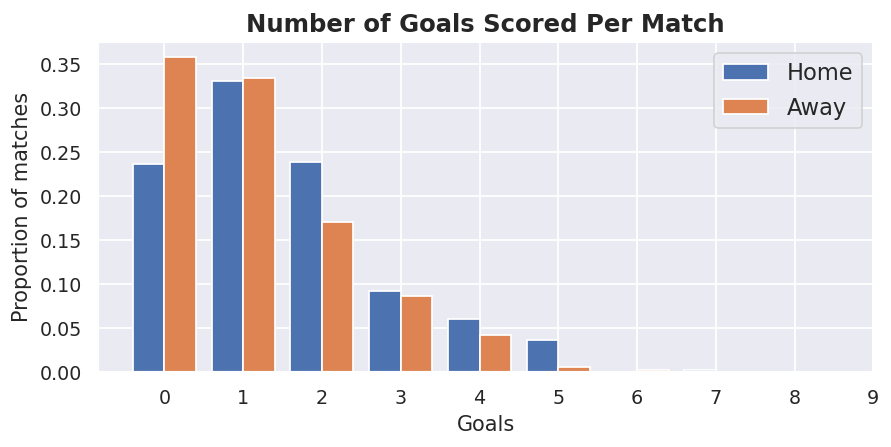
The shape of that distribution looks rather similar to the Poisson distribution. We can confirm this by overlaying the number of goals we'd expect from the Poisson distribution based on the average goals scored that we calculated above.
import numpy as np
from scipy.stats import poisson

home_poisson = poisson.pmf(range(10), df["FTHG"].mean())
away_poisson = poisson.pmf(range(10), df["FTAG"].mean())

max_goals = 10
plt.hist(
    df[["FTHG", "FTAG"]].values, range(max_goals), label=["Home", "Away"], density=True
)

plt.plot(
    [i - 0.5 for i in range(1, max_goals + 1)],
    home_poisson,
    linestyle="-",
    marker="o",
    label="Home Poisson",
)

plt.plot(
    [i - 0.5 for i in range(1, max_goals + 1)],
    away_poisson,
    linestyle="-",
    marker="o",
    label="Away Poisson",
)


plt.xticks([i - 0.5 for i in range(1, max_goals + 1)], [i for i in range(max_goals)])
plt.xlabel("Goals")
plt.ylabel("Proportion of matches")
plt.legend(loc="upper right", fontsize=13)
plt.title("Number of Goals Scored Per Match", size=14, fontweight="bold")
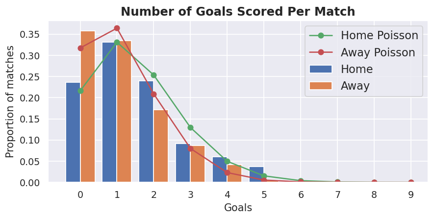
It's not perfect, but the two sets of data look pretty close to each other. This is good as it means we can approximate the number of goals scored using the Poisson distribution - this assumption is going to form the basis of our predictive model.
Building the model
To plot the Poisson distributions above, we used the average number of goals scored home and away, but to predict actual matches we're going to need to know how many goals we expect each individual team to score against each other.
For this, we're going to assume that the number of goals a team scores is a function of their attack strength combined with the opposition's defence strength. In other words, teams with better attacks should score more and teams with worse defences should concede more.
We also need to remember to account for the home advantage too.
So our model is going to look like this:
goals_home = home_advantage + home_attack + defence_away
goals_away = away_attack + defence_home
So far, so good. But where do we get the values for those model parameters from???
We're going to use good old trial and error to test out a whole bunch of different numbers and see what works best. We are not going to do it by hand though as that will be tedious. Instead, we'll let the computer do the hard work for us.
Finding the Optimal parameters
For our computer to find the best set of attack and defence parameters, we need to give it a value to optimise. For a problem like this, the usual approach is Maximum Likelihood Estimation for identifying the parameter values that maximise the likelihood that the process described by the model produces the data that were actually observed. In other words, it will work out what set of attack and defence parameters get closest to reproducing those historical fixtures we downloaded.
Unfortunately, for this example calculating the likelihood involves multiplying lots of small numbers together, which can cause issues with floating point precision and underflows.
Instead, we'll maximise the log-likelihood as we can just sum the logs of the likelihoods togethers rather than multiplying and avoid all those awkward precision issues.
And actually, instead of maximising the log-likelihood, we're going to minimize the negative of the log-likelihood because Python's scipy library comes with an optimizer that minimizes rather than maximizes. If this is confusing, making the negative of the log-likelihood as small as possible is equivalent to making the log-likelihood itself as big as possible.
Now we just need the function to calculate the log- likelihood.
def log_likelihood(
    goals_home_observed,
    goals_away_observed,
    home_attack,
    home_defence,
    away_attack,
    away_defence,
    home_advantage,
):
    goal_expectation_home = np.exp(home_attack + away_defence + home_advantage)
    goal_expectation_away = np.exp(away_attack + home_defence)

    if goal_expectation_home < 0 or goal_expectation_away < 0:
        return 10000

    home_llk = poisson.pmf(goals_home_observed, goal_expectation_home)
    away_llk = poisson.pmf(goals_away_observed, goal_expectation_away)

    log_llk = np.log(home_llk) + np.log(away_llk)

    return -log_llk
That function is less complicated than it initially looks. First, we put the attack, defence and home_advantage parameters into the model we defined above to get the number of goals we expect from the two teams playing each other. If the number of goals is less than zero then we return a really big number to tell the optimizer that the parameters it is testing are rubbish because teams can't score less than zero goals in real life.
If we have zero or more goals, we use the Poisson distribution we work out the likelihood of our parameters giving us the actual number of goals scored. We then convert that to its log and add them together. Finally, because we are minimizing instead of maximizing, we return the negative of the log-likelihood.
Now we need to wrap that code to pass into the optimizer.
from scipy.optimize import minimize


def fit_poisson_model():
    teams = np.sort(np.unique(np.concatenate([df["HomeTeam"], df["AwayTeam"]])))
    n_teams = len(teams)

    params = np.concatenate(
        (
            np.random.uniform(0.5, 1.5, (n_teams)),  # attack strength
            np.random.uniform(0, -1, (n_teams)),  # defence strength
            [0.25],  # home advantage
        )
    )

    def _fit(params, df, teams):
        attack_params = dict(zip(teams, params[:n_teams]))
        defence_params = dict(zip(teams, params[n_teams : (2 * n_teams)]))
        home_advantage = params[-1]

        llk = list()
        for idx, row in df.iterrows():
            tmp = log_likelihood(
                row["FTHG"],
                row["FTAG"],
                attack_params[row["HomeTeam"]],
                defence_params[row["HomeTeam"]],
                attack_params[row["AwayTeam"]],
                defence_params[row["AwayTeam"]],
                home_advantage,
            )
            llk.append(tmp)

        return np.sum(llk)

    options = {
        "maxiter": 100,
        "disp": False,
    }

    constraints = [{"type": "eq", "fun": lambda x: sum(x[:n_teams]) - n_teams}]

    res = minimize(
        _fit,
        params,
        args=(df, teams),
        constraints=constraints,
        options=options,
    )

    model_params = dict(
        zip(
            ["attack_" + team for team in teams]
            + ["defence_" + team for team in teams]
            + ["home_adv"],
            res["x"],
        )
    )

    return model_params

model_params = fit_poisson_model()
That's a big chunk of code so let's step through it to see what it's doing.
First of all, we extract the teams from those historical fixtures we are fitting the model to as we're going to need to use them later on to index into the model's parameters with.
Next, we create the default model parameters. The optimizer will use these as a starting point so the closer we can get them to the actual values then the easier (and therefore quicker) it will be for the optimizer to do its job.
We then create a function called _fit, which is a wrapper around the function for calculating the log-likelihood. This loops through our historical fixtures, calculates the log-likelihood for each one and then adds them all up. It's this final number that the optimizer is using to work out what the best set of parameters is.
Just a small warning here that this function is rather slow. I've tried to keep the code as simple as possible by just using a for loop here but there are ways to rewrite this to speed it up massively, which I'll point you towards later.
We then set up some additional options for the optimizer to tell it to give up if it has not found a solution after 100 attempts and to hide the default output.
Next, we set up a constraint to tell the optimizer that the sum of the attack parameters must equal the total number of teams. There are countless combinations of parameters that could potentially give us the same results so this forces the optimizer to give us a reproducible output and keeps the parameters in a realistic range by making them average around 1.
After all that, we finally run the optimizer and return the parameters it has decided are the best fit.
Let's take a look at the parameters and check they look sensible
from pprint import pprint

pprint(model_params)
{'attack_Arsenal': 1.4472981861257104,
 'attack_Bournemouth': 0.9586519453041221,
 'attack_Brighton': 0.6704348922643556,
 'attack_Burnley': 0.7124518794812125,
 'attack_Chelsea': 1.2560897724037843,
 'attack_Crystal Palace': 0.9524125006581355,
 'attack_Everton': 0.9329845923970115,
 'attack_Huddersfield': 0.4800186720177229,
 'attack_Leicester': 1.1770358138298533,
 'attack_Liverpool': 1.5606892885829151,
 'attack_Man City': 1.782353073898856,
 'attack_Man United': 1.3383146669687525,
 'attack_Newcastle': 0.8007419035953682,
 'attack_Southampton': 0.7572219737186204,
 'attack_Stoke': 0.7139419884005881,
 'attack_Swansea': 0.4779863899533932,
 'attack_Tottenham': 1.4314120522353588,
 'attack_Watford': 0.9392553101070111,
 'attack_West Brom': 0.5799340702765279,
 'attack_West Ham': 1.0307710277807003,
 'defence_Arsenal': -0.904617084909674,
 'defence_Bournemouth': -0.7555648468890336,
 'defence_Brighton': -0.8891290180796632,
 'defence_Burnley': -1.213060870426372,
 'defence_Chelsea': -1.2124734969715354,
 'defence_Crystal Palace': -0.8593840991466305,
 'defence_Everton': -0.8071894597751467,
 'defence_Huddersfield': -0.8236837487885708,
 'defence_Leicester': -0.7605866654074676,
 'defence_Liverpool': -1.1893484944870034,
 'defence_Man City': -1.5087555344502186,
 'defence_Man United': -1.5123413324174197,
 'defence_Newcastle': -1.0231224233993557,
 'defence_Southampton': -0.8496091601384902,
 'defence_Stoke': -0.6570589447421037,
 'defence_Swansea': -0.8588218644055267,
 'defence_Tottenham': -1.254167039595323,
 'defence_Watford': -0.7084540000589359,
 'defence_West Brom': -0.8557753688634717,
 'defence_West Ham': -0.6434205443618255,
 'home_adv': 0.2888264579592506}
That looks reasonable to me, Huddersfield and West Brom both have low attack parameters reflecting that they didn't score many goals while Manchester City and Chelsea have much higher attack parameters. West Ham and Bournemouth both have poor defence parameters, which again matches what actually happened in our historical data.
Our home advantage parameter is also pretty close to what we got by just looking at the difference in average goals scored home and away.
Predicting Scores
Now for the fun bit, let's start making some predictions :)
def predict(home_team, away_team, params, max_goals=10):
    home_attack = params["attack_" + home_team]
    home_defence = params["defence_" + home_team]
    away_attack = params["attack_" + away_team]
    away_defence = params["defence_" + away_team]
    home_advantage = params["home_adv"]

    home_goal_expectation = np.exp(home_attack + away_defence + home_advantage)
    away_goal_expectation = np.exp(away_attack + home_defence)

    home_probs = poisson.pmf(list(range(max_goals + 1)), home_goal_expectation)
    away_probs = poisson.pmf(range(max_goals + 1), away_goal_expectation)

    probability_matrix = np.outer(home_probs, away_probs)

    return probability_matrix
The start of this function looks similar to the log_likelihood function we used when fitting the model. We start off by getting the parameters and using them to calculate how many goals we expect the home and away team to score against each other.
We then use that with the Poisson distribution to get the probability of each team scoring 0, 1, 2, 3 etc goals.
Then take the outer product of those two sets of probabilities to get a matrix containing the probability of all the possible scores.
Let's give it a go and get the probabilities for all scores up to four goals!
probs = predict("Man City", "Stoke", model_params, 4)
pprint(probs)
array([[0.01041474, 0.00470398, 0.00106231, 0.00015994, 0.00001806],
       [0.04283444, 0.01934684, 0.00436915, 0.0006578 , 0.00007428],
       [0.0880862 , 0.03978549, 0.00898487, 0.00135272, 0.00015274],
       [0.1207623 , 0.05454416, 0.01231786, 0.00185452, 0.00020941],
       [0.12416985, 0.05608323, 0.01266543, 0.00190685, 0.00021531]])
The columns show the probability of Manchester City scoring a given number of goals, whilst the rows are the probabilities for Stoke. For example, the probability of 0-0 is 0.01041474 and the probability of 3-1 is 0.05454416.
We can now use this matrix to get the probabilities for various betting markets. For example, the sum of the diagonal of the matrix gives us the probability of a draw, the sum of the lower triangle is the probability of a home win and the sum of the upper triangle is the probability of an away win.
# draw
np.sum(np.diag(probs))
0.04081627039389976
# home win
np.sum(np.tril(probs, -1))
0.5531558007746874
# away win
np.sum(np.triu(probs, 1))
0.01276037463224738
Note that those probabilities don't add up to one as we've only calculated the probabilities for up to 4 goals. By the time you get up to 10 goals then you're pretty much at 1.0.
Something Smells a Bit Fishy
We now have a model and can make predictions but are those predictions any good??
If we look at the average probabilities over our data set then our model expects around 46% of games to finish as a home win, 23% as a draw and 31% as an away win.
However, if we look at what actually happened that season then 46% of games ended as a home win, 26% as a draw and 28% as an away win - that's pretty good but we're clearly under-predicting draws and over-predicting away wins. If you're planning on using this model to beat the bookie then you're likely to be disappointed at this stage.
The problem is that we're predicting the number of goals each team scores independently from each other. But goals in a football match are not independent. For example, the team playing away may settle for a draw if the game is 0-0 in the second half and attack less. A team that's gone three goals down may park the bus to try and avoid a more humiliating score line.
So there are situations where teams aren't necessarily playing to score and that negatively impacts our Poisson assumption.
Conclusions
All of this is not to say our model is useless though, it actually gives us a really good base model to build upon.
In the next article in this series, we'll look at how Dixon and Coles propose an adjustment to our Poisson model to try and alleviate these issues with under-predicting draws and improve our accuracy.
Addendum
I mentioned above that the function we were using to optimize was a little slow as the code was written for simplicity rather than speed.
I've neatened up the code and added it my penaltyblog python package if you want to try out a faster version. This package also includes some other useful functions for working with football and betting data.
It's as simple as:
pip install penaltyblog
df = pb.footballdata.fetch_data("England", 2017, 0)
df[["Date", "HomeTeam", "AwayTeam", "FTHG", "FTAG"]].head()

pois = pb.poisson.PoissonGoalsModel(df["FTHG"], df["FTAG"], df["HomeTeam"], df["AwayTeam"])
pois.fit()
probs = pois.predict("Man City", "Man United")
print(probs.home_draw_away)
[0.5645798158431763, 0.23488303272721173, 0.20053715077601225]
Have fun!